GBDT 基本概述

概述

GBDT 是 Gradient Boosting Decision Tree 的缩写，属于集成学习方法中的 Boosting 族。

它的核心思想是通过逐步构成多个决策树，每棵树都试图纠正前一棵树的残差，最终所有树的结果相加得到最终预测结果

这里的关键点在于如何通过梯度下降来最小化损失函数，从而确定每棵树的参数

梯度提升的一般步骤

初始化模型，通常一个常数，比如所有样本的均值(对于回归问题)
计算当前模型的残差(即负梯度)
用决策树拟合这些残差
更新模型，将新树的预测结果乘以一个学习率加到原有模型上
重复步骤2-4，直到达到预设树的数量或残差足够小

GBDT 的数学框架

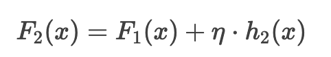
GBDT 是加法模型，通过迭代训练M棵决策树(基学习器)，最终模型为:
在这里插入图片描述

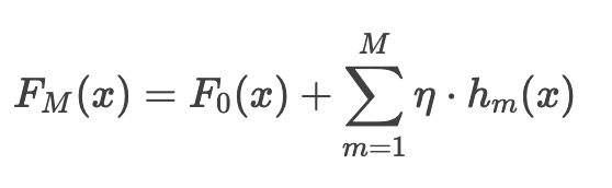
其中:

F0(x) 是初始模型(常取目标均值)
hm(x) 是第m棵树的预测值
η 是学习率(步长)，控制每棵树的贡献

核心步骤

初始化模型:

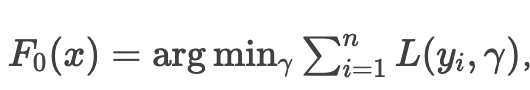
通常取目标值的均值

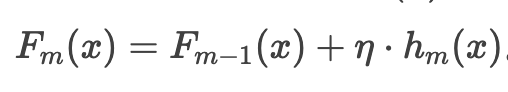
迭代提升
对于每棵树 m = 1,2,…,M:

计算当前模型的负梯度(残差近似值)
用决策树拟合负梯度, 得到树结构 hm(x)
更新模型:

实例说明: 回归问题

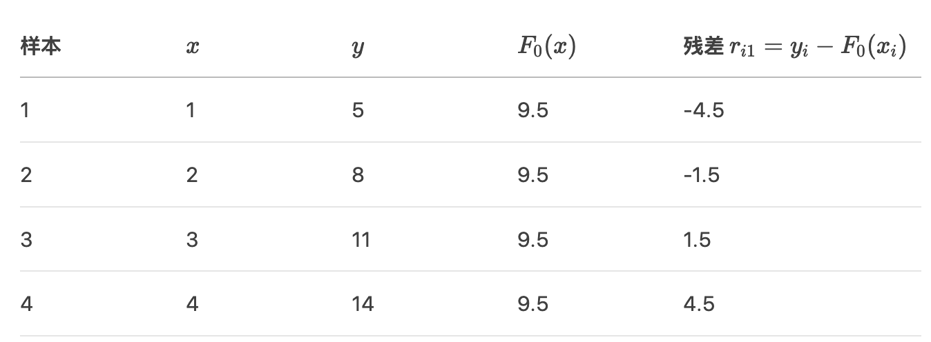
假设训练数据如下: (4个样本，特征x，目标y)

在这里插入图片描述

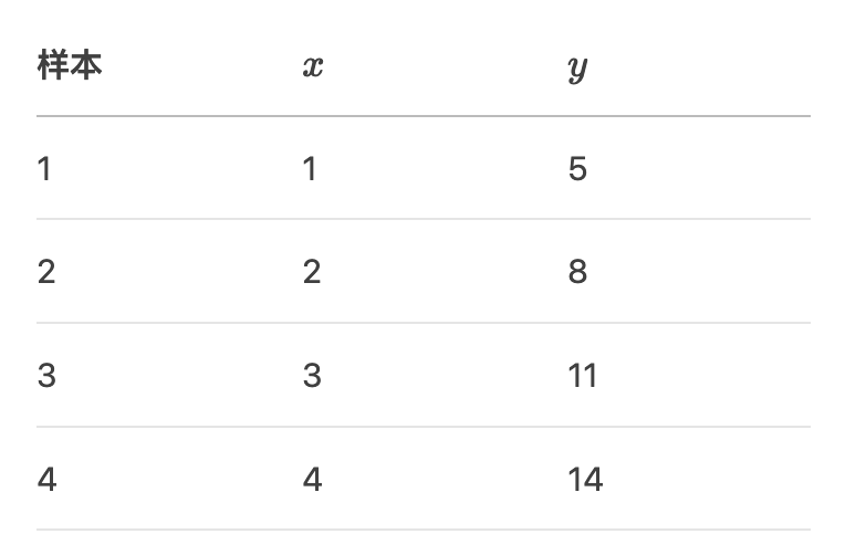
目标: 用GBDT 拟合 y = 3x + 2的线性关系(实际应用中GBDT 常用于非线性关系，此处用于简化)

第1步: 初始化模型 F0(x)

初始模型通常为目标值的均值:
在这里插入图片描述

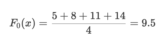
此时所有样本的预测值均为9.5

第2步：第1棵树(m = 1)

1. 计算残差(负梯度)

对于平均损失函数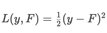在这里插入图片描述

, 负梯度:
在这里插入图片描述

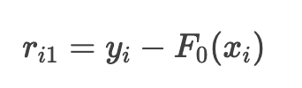
各样本的残差:
在这里插入图片描述

2. 用决策树拟合残差

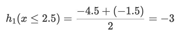
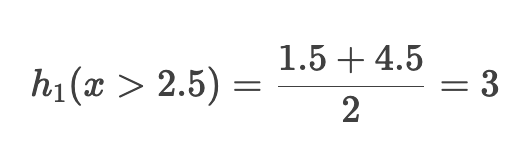
假设我们生成一个深度为1的树(即单层分裂): 分裂点为 x <= 2.5:

左叶子节点 (x <= 2.5。样本1和2)的预测值:
在这里插入图片描述

右叶子节点 (x > 2.5，样本3和4)的预测值：
在这里插入图片描述

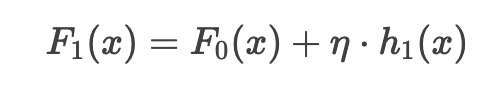
3. 更新模型

假设学习率 η = 0.1 ,更新后的模型:
在这里插入图片描述

各样本预测值:

样本1和2: 9.5 + 0.1 * (-3) = 9.2
样本3和4: 9.5 + 0.1 * 3 = 9.8

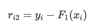
第3步: 第2棵树(m = 2)

1. 计算新的残差

当前预测值 F1(x) 与真实值的残差：
在这里插入图片描述

在这里插入图片描述

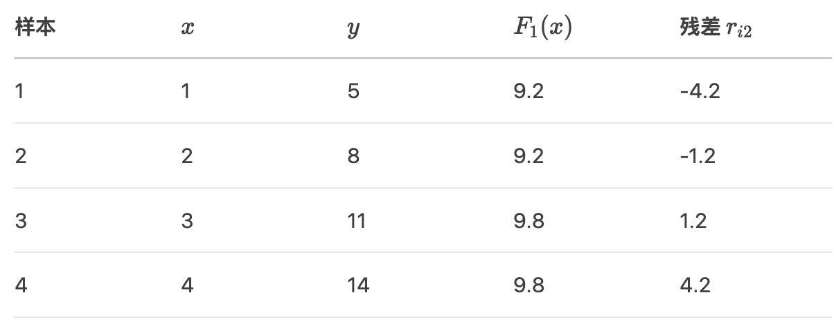
2. 用决策树拟合新残差

同样使用深度1的树，分裂点仍为 x <= 2.5

左叶子节点预测值: (-4.2 - 1.2) / 2 = -2.7
右叶子节点预测值: (1.2 + 4.2) / 2 = 2.7

3. 更新模型

在这里插入图片描述

各样本预测值:

样本1和2： 9.2 + 0.1 * （-2.7）= 8.93
样本3和4: 9.8 + 0.1 * 2.7 = 10.07

迭代继续

重复上述步骤，每一棵树都在拟合当前模型的残差。经过多轮迭代后，预测值逐渐逼近真实值

案例

Python 实现 Boosting Tree

from collections import defaultdict
import numpy as npclass BoostingTree:def __init__(self, error=1e-2):self.error = error # 误差值self.candidate_splits = [] # 候选切分点self.split_index = defaultdict(tuple) # 由于要多次切分数据集，故预先存储，切分后数据点的索引self.split_list = [] # 最终各个基本回归树的切分点self.c1_list = [] # 切分点左区域取值（均值）self.c2_list = [] # 切分点右区域取值（均值）self.N = None # 数组元素个数self.n_split = None # 切分点个数# 切分数组函数def split_arr(self, X_data):self.N = X_data.shape[0]# 候选切分点——前后两个数的中间值for i in range(1, self.N):self.candidate_splits.append((X_data[i][0] + X_data[i - 1][0]) / 2)self.n_split = len(self.candidate_splits)# 切成两部分for split in self.candidate_splits:left_index = np.where(X_data[:, 0] <= split)[0]right_index = np.where(X_data[:, 0] > split)[0]self.split_index[split] = (left_index, right_index)return# 计算每个切分点的误差def calculate_error(self, split, y_result):indexs = self.split_index[split]left = y_result[indexs[0]]right = y_result[indexs[1]]c1 = np.sum(left) / len(left)  # 左均值c2 = np.sum(right) / len(right) # 右均值y_result_left = left - c1y_result_right = right - c2result = np.hstack([y_result_left, y_result_right]) # 数据拼接result_square = np.apply_along_axis(lambda x: x ** 2, 0, result).sum()return result_square, c1, c2# 获取最佳切分点，并返回对应的残差def best_split(self, y_result):# 默认第一个为最佳切分点best_split = self.candidate_splits[0]min_result_square, best_c1, best_c2 = self.calculate_error(best_split, y_result)for i in range(1, self.n_split):result_square, c1, c2 = self.calculate_error(self.candidate_splits[i], y_result)if result_square < min_result_square:best_split = self.candidate_splits[i]min_result_square = result_squarebest_c1 = c1best_c2 = c2self.split_list.append(best_split)self.c1_list.append(best_c1)self.c2_list.append(best_c2)return# 基于当前组合树，预测X的输出值def predict_x(self, X):s = 0for split, c1, c2 in zip(self.split_list, self.c1_list, self.c2_list):if X < split:s += c1else:s += c2return s# 每添加一颗回归树，就要更新y,即基于当前组合回归树的预测残差def update_y(self, X_data, y_data):y_result = []for X, y in zip(X_data, y_data):y_result.append(y - self.predict_x(X[0]))  # 残差y_result = np.array(y_result)print(np.round(y_result,2)) # 输出每次拟合训练数据的残差res_square = np.apply_along_axis(lambda x: x ** 2, 0, y_result).sum()return y_result, res_squaredef fit(self, X_data, y_data):self.split_arr(X_data)y_result = y_datawhile True:self.best_split(y_result)y_result, result_square = self.update_y(X_data, y_data)if result_square < self.error:breakreturndef predict(self, X):return self.predict_x(X)if __name__ == '__main__':data = np.array([[1, 5.56], [2, 5.70], [3, 5.91], [4, 6.40], [5, 6.80],[6, 7.05], [7, 8.90], [8, 8.70], [9, 9.00], [10, 9.05]])X_data = data[:, :-1]y_data = data[:, -1]bt = BoostingTree(error=0.18)bt.fit(X_data, y_data)print('切分点：', bt.split_list)print('切分点左区域取值:', np.round(bt.c1_list,2))print('切分点右区域取值:', np.round(bt.c2_list,2))

结果:

[-0.68 -0.54 -0.33  0.16  0.56  0.81 -0.01 -0.21  0.09  0.14]
[-0.16 -0.02  0.19 -0.06  0.34  0.59 -0.23 -0.43 -0.13 -0.08]
[-0.31 -0.17  0.04 -0.2   0.2   0.45 -0.01 -0.21  0.09  0.14]
[-0.15 -0.01  0.2  -0.04  0.09  0.34 -0.12 -0.32 -0.02  0.03]
[-0.22 -0.08  0.13 -0.11  0.02  0.27 -0.01 -0.21  0.09  0.14]
[-0.07  0.07  0.09 -0.15 -0.02  0.23 -0.05 -0.25  0.05  0.1 ]
切分点： [6.5, 3.5, 6.5, 4.5, 6.5, 2.5]
切分点左区域取值: [ 6.24 -0.51  0.15 -0.16  0.07 -0.15]
切分点右区域取值: [ 8.91  0.22 -0.22  0.11 -0.11  0.04]