目录
效果前瞻
建模
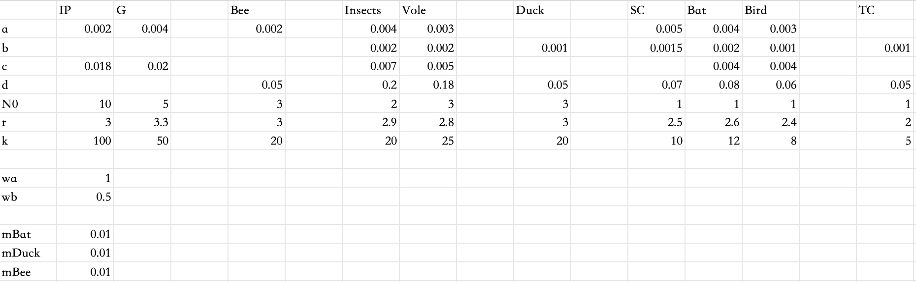
参数表
构图
饼图
二维敏感性
极坐标柱状图
季节敏感性
斯皮尔曼相关矩阵
各微调模型的敏感性分析
技术栈:Python(Matplotlib、Seaborn、Numpy、Pandas、Scipy)、动态系统模拟(Euler 方法)、时间序列分析
更多数据可视化的代码可以参考数模13种可视化脚本-Python-CSDN博客
效果前瞻
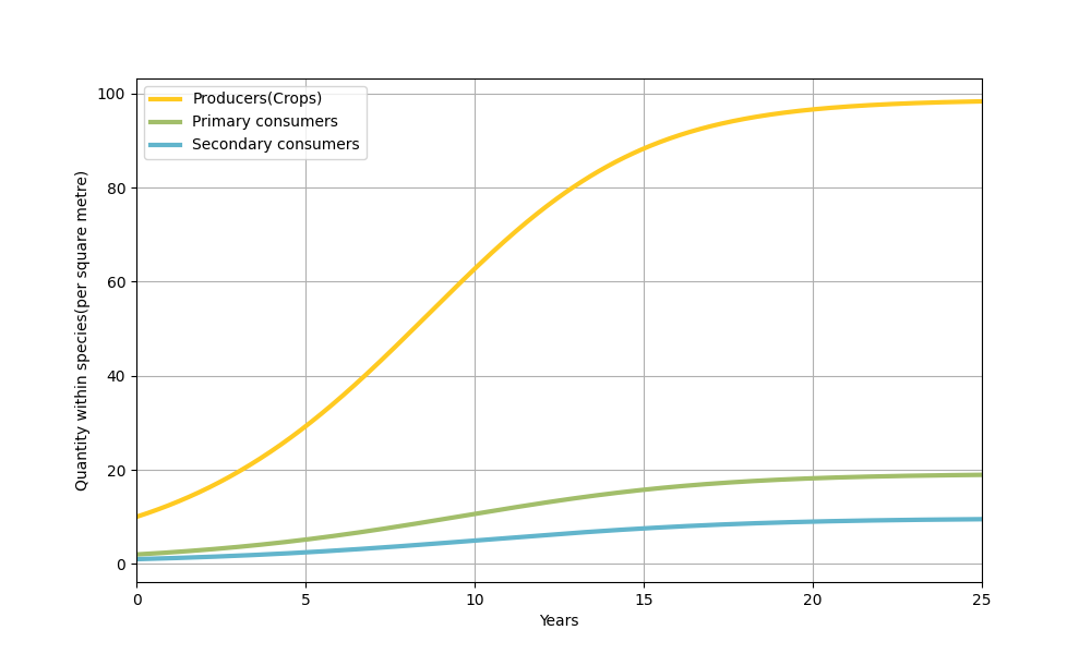
基准模型三阶层图

饼图
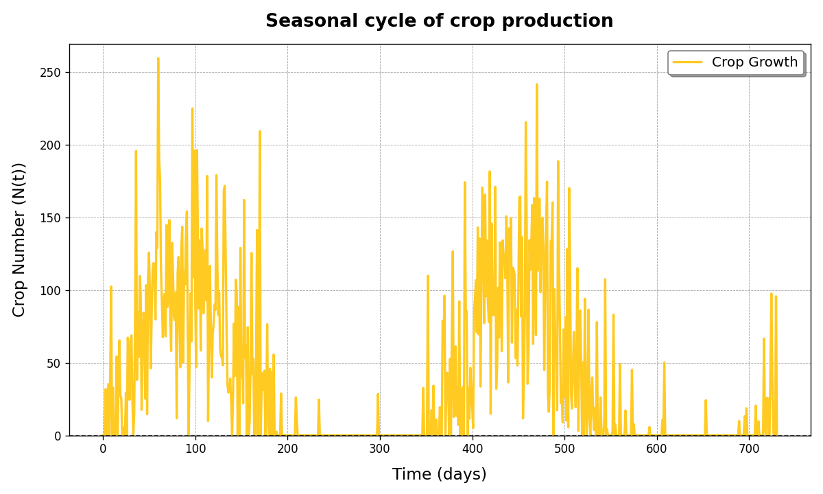
季节性
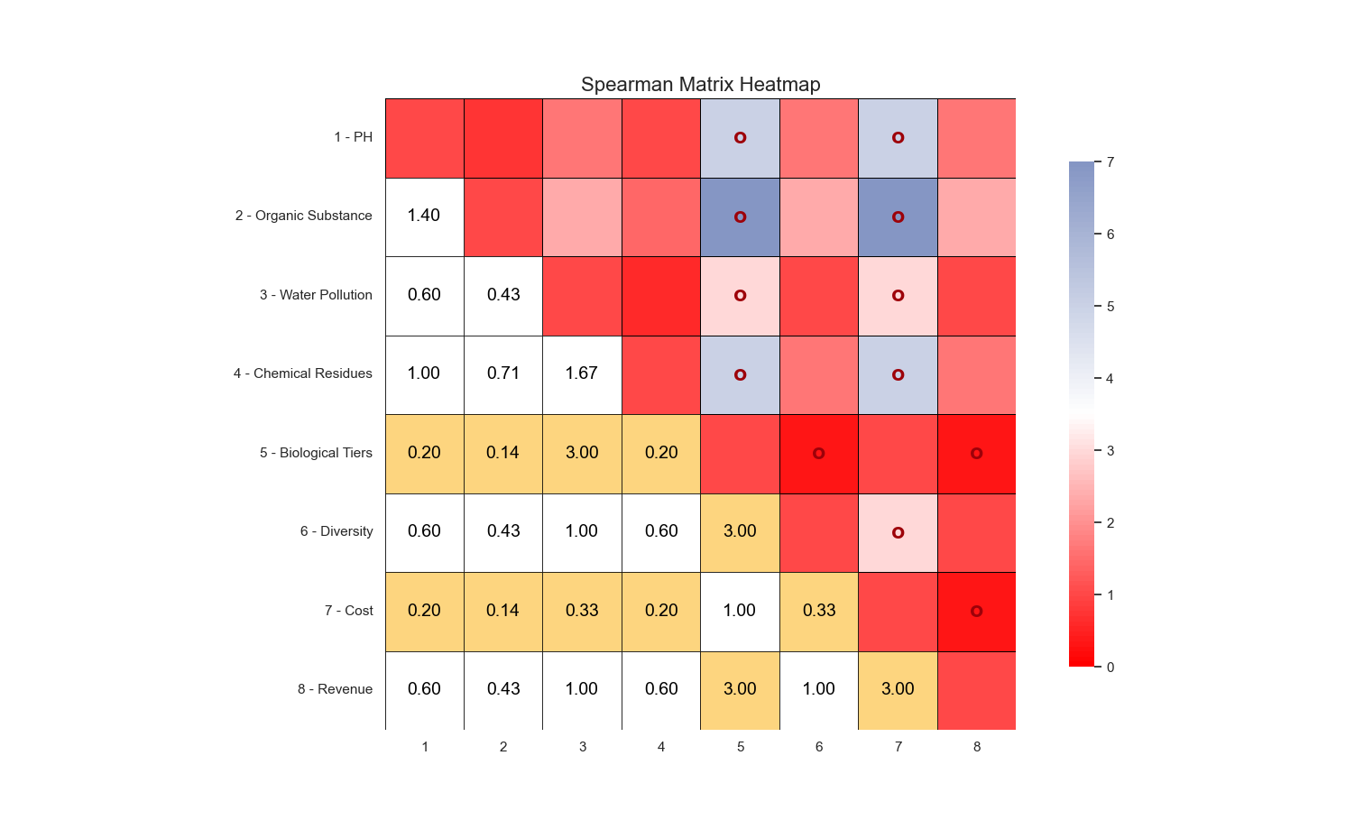
相关矩阵
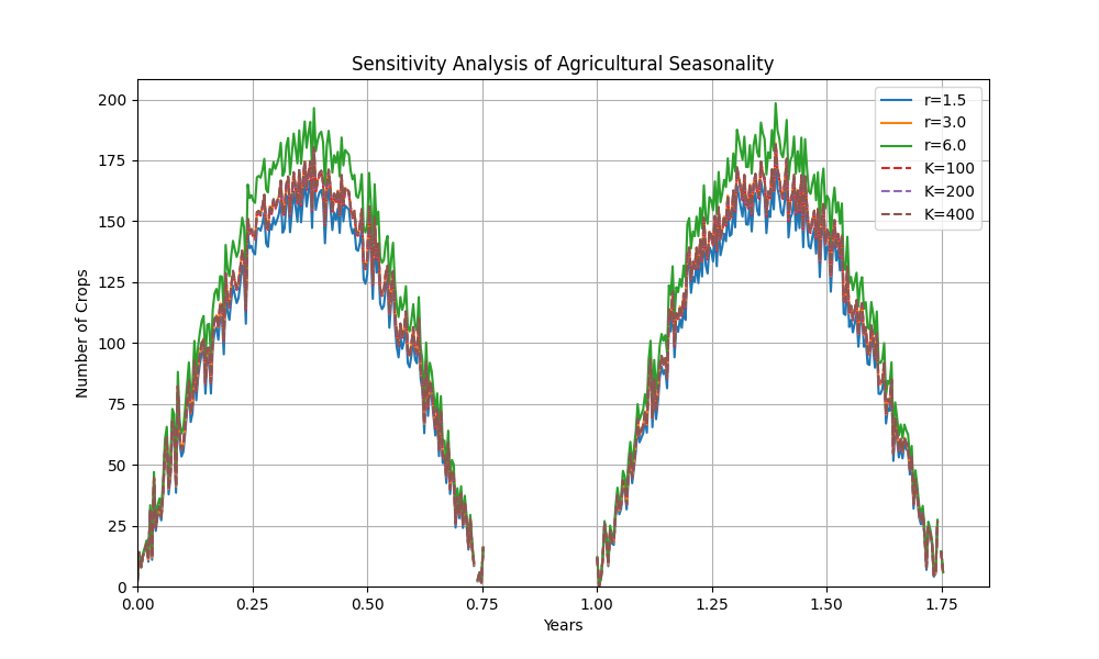
季节敏感性分析
各微调模型的敏感性分析
建模
根据LV方程对基准模型进行分层,用Euler方法进行模拟
对于不同阶段的模型,都是在这个基准模型的基础上进行微调
import numpy as np
import matplotlib.pyplot as plt
from matplotlib import font_manager
from scipy.interpolate import make_interp_spline#受下层食物限制系数    角标
aP=0.002aI=0.004aS=0.005#捕食系数和a一个数量级bI=0.002bS=0.001
bBat=0.002
bBird=0.001#竞争系数       #a、b、c同一量级
cP=0.018
cG=0.02  #杂草的竞争系数比农作物的大cI=0.007cBat=0.5
cBird=0.2#自然死亡 相较于a、b应该多一个I的数量级    昆虫>鸟>蝙蝠
dI,dS=0.1,0.07
dBat,dBird=0.8,0.6#化学影响 相较于a、b应该多一个I的数量级
wa=1     #除草
wb=0.5     #除虫#传播
#mBat=#初始数量    10:5:2:1
P0,G0,I0,I20,S0=10,5,2,2,1
Bat0,Bird0=1,1#自然增长   昆虫极大>鸟>蝙蝠
rP,rG,rI,rS=3,3.3,2.7,2.5
rBat,rBird=3.3,2.7#限制 公顷
kP,kG,kI,kS=100,50,20,10
kBat,kBird=10,10#设置时长和最大时间
dt=1     #步长
T=25    #总时间
time_steps=int(T/dt)        #总步数#初始化数量数组
P=np.zeros(time_steps)
G=np.zeros(time_steps)
I=np.zeros(time_steps)
S=np.zeros(time_steps)P[0], G[0], I[0], S[0] = P0,G0,I0, S0  # 初始化数量#层级化
def P0(t):return rP*(1-P[t-1]/kP)*P[t-1]          -bI*I[t-1]*P[t-1]
def G0(t):#杂草0:只考虑了自然生长return rG*(1-G[t-1]/kG)*G[t-1]def I0(t):return rI*(1-I[t-1]/kI)*I[t-1]-dI*I[t-1]-bS*S[t-1]*I[t-1]-aP*I[t-1]def S0(t):return rS*(1-S[t-1]/kS)*S[t-1]-dS*S[t-1]                 -aI*S[t-1]#第一问:分第一层,不分第三层
for t in range(1,time_steps):DP=P0(t)    #竟然将dp!!!!再次定义!导致。。#DG=G0(t)-cP*P[t-1]*G[t-1]-wa*G[t-1]DI=I0(t)DS=S0(t)#更新每个物种数量P[t]=(P[t-1]+DP*dt/10)#G[t]=(G[t-1]+DG*dt/10)I[t]=(I[t-1]+DI*dt/10)S[t]=(S[t-1]+DS*dt/10)print(P[-1])
print(G[-1])
print(I[-1])
print(S[-1])# 时间序列
time = np.linspace(0, T, time_steps)# 对每个物种进行插值
smooth_time = np.linspace(0, T, 500)  # 更高分辨率的时间序列
P_smooth = make_interp_spline(time, P)(smooth_time)
#G_smooth = make_interp_spline(time, G)(smooth_time)
I_smooth = make_interp_spline(time, I)(smooth_time)
S_smooth = make_interp_spline(time, S)(smooth_time)# 绘制平滑曲线
plt.figure(figsize=(10, 6))
plt.plot(smooth_time, P_smooth, label='Producers(Crops)', color='#FFCA21', linewidth=3)
#plt.plot(smooth_time, G_smooth, label='Weeds', color='#D5BE98', linewidth=3)
plt.plot(smooth_time, I_smooth, label='Primary consumers', color='#A2BE6A', linewidth=3)
plt.plot(smooth_time, S_smooth, label='Secondary consumers', color='#62B5CC', linewidth=3)
plt.legend()
plt.xlabel('Years')
plt.ylabel('Quantity within species(per square metre)')
#plt.title('Ecosystem population dynamics')# 去除x轴两端留白
plt.xlim(0, T)'''
# 设置x轴刻度间隔为1
plt.xticks(np.arange(0, T + 1, 1))'''
plt.grid(True)
plt.show()
参数表
构图
饼图
from pyecharts import options as opts
from pyecharts.charts import Pie# 创建 Pie 实例
pie = Pie()# 添加数据
pie.add(series_name="Example",data_pair=[("A", 40), ("B", 30), ("C", 20), ("D", 10)],radius=["30%", "70%"],  # 设置内外半径,创建环形效果label_opts=opts.LabelOpts(is_show=True)  # 显示标签
)# 设置颜色
pie.set_global_opts(legend_opts=opts.LegendOpts(is_show=True),  # 显示图例toolbox_opts=opts.ToolboxOpts(is_show=True)  # 工具栏
).set_series_opts(itemstyle_opts=opts.ItemStyleOpts(color="#FF5733")  # 设置颜色
)# 渲染图表
pie.render("filled_pie_chart.html")
二维敏感性
import numpy as np
import matplotlib.pyplot as plt
import seaborn as sns# 固定的参数
aP, aI, aI2, aS, aBat, aBird = 0.002, 0.004, 0.004, 0.005, 0.005, 0.005
bI, bI2, bS, bBat, bBird, bF = 0.002, 0.002, 0.001, 0.002, 0.001, 0.001
cP, cG, cI, cI2, cBat, cBird = 0.018, 0.02, 0.007, 0.005, 0.004, 0.004
dI, dI2, dS, dBat, dBird, dF = 0.2, 0.18, 0.07, 0.08, 0.06, 0.05
wa, wb = 1, 0.5
P0, G0, I0, I20, S0, Bat0, Bird0, F0 = 10, 5, 2, 3, 1, 1, 1, 1
rP, rG, rI, rI2, rS = 3, 3.3, 2.9, 2.8, 2.5
rBat, rBird, rF = 2.6, 2.4, 2
kP, kG, kI, kI2, kS = 100, 50, 20, 25, 10
kBat, kBird, kF = 10, 8, 5# 时间设置
dt = 0.1
T = 12
time_steps = int(T / dt)# 种群初始化
P = np.zeros(time_steps)
G = np.zeros(time_steps)
I = np.zeros(time_steps)
S = np.zeros(time_steps)
F = np.zeros(time_steps)# 定义种群变化函数
def P0_func(t):return rP * (1 - P[t-1] / kP) * P[t-1] - bI * I[t-1] * P[t-1]def G0_func(t):return rG * (1 - G[t-1] / kG) * G[t-1]def I0_func(t):return rI * (1 - I[t-1] / kI) * I[t-1] - dI * I[t-1] - bS * S[t-1] * I[t-1] - aP * P[t-1] * I[t-1]def S0_func(t):return rS * (1 - S[t-1] / kS) * S[t-1] - dS * S[t-1] - aI * I[t-1] * S[t-1]# 参数范围
param_ranges = {"rP": np.linspace(rP * 0.9, rP * 1.1, 20),"kP": np.linspace(kP * 0.9, kP * 1.1, 20),"dP": np.linspace(dI * 0.9, dI * 1.1, 20),
}# 热力图计算函数
def compute_heatmap(param1_name, param2_name):param1_values = param_ranges[param1_name]param2_values = param_ranges[param2_name]param1_grid, param2_grid = np.meshgrid(param1_values, param2_values)results = np.zeros_like(param1_grid)for i in range(param1_grid.shape[0]):for j in range(param1_grid.shape[1]):globals()[param1_name] = param1_grid[i, j]globals()[param2_name] = param2_grid[i, j]# 初始化种群P[:] = P0G[:] = G0I[:] = I0S[:] = S0F[:] = F0# 模拟for t in range(1, time_steps):DP = P0_func(t)DG = G0_func(t)DI = I0_func(t)DS = S0_func(t)DF = rF * (1 - F[t-1] / kF) - dF * F[t-1]P[t] = P[t-1] + DP * dt / 5G[t] = G[t-1] + DG * dt / 5I[t] = I[t-1] + DI * dt / 5S[t] = S[t-1] + DS * dt / 5F[t] = F[t-1] + DF * dt / 5results[i, j] = P[-1]  # 最终作物数量return param1_grid, param2_grid, results# 绘制热力图函数
def plot_heatmap(param1_name, param2_name, title):param1_grid, param2_grid, results = compute_heatmap(param1_name, param2_name)plt.figure(figsize=(8, 6))sns.heatmap(results, xticklabels=np.round(param_ranges[param1_name], 2),yticklabels=np.round(param_ranges[param2_name], 2), cmap="viridis", cbar_kws={'label': 'Final Crop Quantity'})plt.title(title)plt.xlabel(param1_name)plt.ylabel(param2_name)plt.show()# 绘制单独的热力图
plot_heatmap("rP", "kP", "Sensitivity: rP vs kP")
plot_heatmap("kP", "dP", "Sensitivity: kP vs dP")
plot_heatmap("dP", "rP", "Sensitivity: dP vs rP")
极坐标柱状图
from pyecharts import options as opts
from pyecharts.charts import Polar# 创建 Polar 实例
polar = Polar()# 添加数据
polar.add(series_name="A",data=[1, 2, 3, 4],type_="bar",  # 设置为极坐标柱状图stack="a",  # 数据堆叠label_opts=opts.LabelOpts(is_show=True),  # 显示标签
)
polar.add(series_name="B",data=[2, 4, 6, 8],type_="bar",stack="a",label_opts=opts.LabelOpts(is_show=True),
)
polar.add(series_name="C",data=[1, 2, 3, 4],type_="bar",stack="a",label_opts=opts.LabelOpts(is_show=True),
)# 配置极坐标的坐标轴
polar.add_schema(angleaxis_opts=opts.AngleAxisOpts(),  # 设置角度轴radiusaxis_opts=opts.RadiusAxisOpts(  # 设置半径轴type_="category",data=["Mon", "Tue", "Wed", "Thu"])
)# 设置全局配置
polar.set_global_opts(legend_opts=opts.LegendOpts(is_show=True),  # 显示图例toolbox_opts=opts.ToolboxOpts(is_show=True)  # 工具栏
)# 渲染图表
polar.render("polar_bar_chart.html")
季节敏感性
import numpy as np
import matplotlib.pyplot as plt# 定义公式参数
N0 = 10        # 初始值
r = 0.1       # 增长率
K = 200        # 环境容量
T = 3/2         # 周期
time = np.linspace(0, 3.5, 1000)  # 时间范围
epsilon = np.random.normal(0, 0.5, len(time))  # 噪声# 定义函数 N(t)
def N(t, N0, r, K, T, epsilon):result = N0 * np.exp(r * (1 - N0 / K)) * np.sin(2 * np.pi * t / T) + epsilon'''if t<1:result = N0 * np.exp(r * (1 - N0 / K)) * np.sin(2 * np.pi * t / T) + epsilonelif t>1.5:return'''result[result <= 0] = np.nan  # 过滤掉 y <= 0 的部分return result*15# 计算 N(t)
N_values = N(time, N0, r, K, T, epsilon)# 绘制敏感性分析(调整参数 r 和 K)
plt.figure(figsize=(10, 6))# r 敏感性分析
for r_test in [0.05, 0.1, 0.2]:N_values_r = N(time, N0, r_test, K, T, epsilon)plt.plot(time, N_values_r, label=f"r={r_test*30}")# K 敏感性分析
for K_test in [100, 200, 400]:N_values_K = N(time, N0, r, K_test, T, epsilon)plt.plot(time, N_values_K, linestyle="--", label=f"K={K_test}")plt.title("Sensitivity Analysis of Agricultural Seasonality")
plt.xlabel("Time")
plt.ylabel("Number of Crops")
plt.legend()
plt.grid()
plt.show()
斯皮尔曼相关矩阵
import pandas as pd
import numpy as np
import seaborn as sns
import matplotlib.pyplot as plt
from matplotlib.colors import LinearSegmentedColormap# 输入8x8矩阵数据
data_array = np.array([[1,5/7,5/3,1,5,5/3,5,5/3],[7/5,1,7/3,7/5,7,7/3,7,7/3],[3/5,3/7,1,3/5,3,1,3,1],[1,5/7,5/3,1,5,5/3,5,5/3],[1/5,1/7,3,1/5,1,1/3,1,1/3],[3/5,3/7,1,3/5,3,1,3,1],[1/5,1/7,1/3,1/5,1,1/3,1,1/3],[3/5,3/7,1,3/5,3,1,3,1]
])# 转换为 DataFrame 格式
data = pd.DataFrame(data_array,columns=[f"Var{i+1}" for i in range(8)],  # 设置列名index=[f"Var{i+1}" for i in range(8)]  # 设置行名
)# 计算斯皮尔曼相关矩阵
corr_matrix = data.corr(method='spearman')# 创建掩码矩阵
mask = np.triu(np.ones_like(corr_matrix, dtype=bool))  # 上三角掩码# 设置绘图风格
plt.figure(figsize=(10, 8))
sns.set_theme(style="white")# 绘制左下部分(数值,无填充颜色,黑色分割线)
sns.heatmap(corr_matrix,mask=mask,  # 显示左下部分annot=True,  # 显示相关系数数值fmt=".2f",  # 数值保留两位小数cmap="coolwarm",  # 使用渐变色,但透明vmin=-1, vmax=1,  # 设置颜色范围cbar=False,  # 不显示颜色条linewidths=0.5,  # 方块分割线宽度linecolor="black",  # 分割线颜色为黑色square=True,  # 方形格子annot_kws={"size": 10},  # 设置字体大小alpha=0  # 左下部分背景透明
)# 自定义配色:蓝黑色到红色渐变
custom_cmap = LinearSegmentedColormap.from_list("blue_black_red", ["red", "white", "#00008B"]  # 蓝黑色到红色渐变
)# 绘制右上部分(颜色渐变,有黑色分割线)
sns.heatmap(corr_matrix,mask=~mask,  # 显示右上部分cmap=custom_cmap,  # 自定义渐变色vmin=0, vmax=7,  # 设置颜色范围cbar_kws={"shrink": 0.8},  # 调整颜色条大小linewidths=0.5,  # 方块分割线宽度linecolor="black",  # 分割线颜色为黑色square=True,  # 方形格子annot=False  # 不显示数值
)# 添加标题
plt.title("Spearman Correlation Matrix", fontsize=16)
plt.show()
各微调模型的敏感性分析
import numpy as np
import matplotlib.pyplot as plt
import seaborn as sns# 上层食物限制系数
aP, aI, aI2, aS, aBat, aBird = 0.002, 0.004, 0.004, 0.005, 0.005, 0.005# 捕食系数和 a 一个数量级
bI, bI2, bS, bBat, bBird, bF = 0.002, 0.002, 0.001, 0.002, 0.001, 0.001# 竞争系数
cP, cG, cI, cI2, cBat, cBird = 0.018, 0.02, 0.007, 0.005, 0.004, 0.004# 自然死亡
dI, dI2, dS, dBat, dBird, dF = 0.2, 0.18, 0.07, 0.08, 0.06, 0.05# 化学影响
wa, wb = 1, 0.5# 初始数量
P0, G0, I0, I20, S0, Bat0, Bird0, F0 = 10, 5, 2, 3, 1, 1, 1, 1# 自然增长
rP, rG, rI, rI2, rS = 3, 3.3, 2.9, 2.8, 2.5
rBat, rBird, rF = 2.6, 2.4, 2# 限制
kP, kG, kI, kI2, kS = 100, 50, 20, 25, 10
kBat, kBird, kF = 10, 8, 5# 设置时长和最大时间
dt = 0.1 # 步长
T = 12 # 总时间
time_steps = int(T / dt) # 总步数# 初始化数量数组
P = np.zeros(time_steps)
G = np.zeros(time_steps)
I = np.zeros(time_steps)
I2 = np.zeros(time_steps)
S = np.zeros(time_steps)
F = np.zeros(time_steps)# 初始化种群
P[0], G[0], I[0], I2[0], S[0], F[0] = P0, G0, I0, I20, S0, F0# 定义种群变化函数
def P0_func(t):return rP * (1 - P[t-1] / kP) * P[t-1] - bI * I[t-1] * P[t-1]def G0_func(t):return rG * (1 - G[t-1] / kG) * G[t-1]def I0_func(t):return rI * (1 - I[t-1] / kI) * I[t-1] - dI * I[t-1] - bS * S[t-1] * I[t-1] - aP * P[t-1] * I[t-1]def S0_func(t):return rS * (1 - S[t-1] / kS) * S[t-1] - dS * S[t-1] - aI * I[t-1] * S[t-1]# 参数范围
rP_values = np.linspace(rP * 0.9, rP * 1.1, 20) # rP 在 ±10% 的范围
kP_values = np.linspace(kP * 0.9, kP * 1.1, 20) # kP 在 ±10% 的范围# 创建网格
rP_grid, kP_grid = np.meshgrid(rP_values, kP_values)# 初始化存储最终结果的数组
final_crops = np.zeros_like(rP_grid)# 遍历参数网格
for i in range(rP_grid.shape[0]):for j in range(rP_grid.shape[1]):rP = rP_grid[i, j] # 当前 rPkP = kP_grid[i, j] # 当前 kP# 重置种群初始值P[:] = P0G[:] = G0I[:] = I0I2[:] = I20S[:] = S0F[:] = F0# 模拟模型for t in range(1, time_steps):DP = P0_func(t) - cG * G[t-1] * P[t-1] - bI2 * I2[t-1] * P[t-1]DG = G0_func(t) - cP * P[t-1] * G[t-1] - wa * G[t-1]DI = I0_func(t) - wb * I[t-1] + bS * S[t-1] * I[t-1]DS = S0_func(t) - aI * I[t-1] * S[t-1] - bF * F[t-1] * S[t-1]DF = rF * (1 - F[t-1] / kF) - dF * F[t-1]# 更新数量P[t] = P[t-1] + DP * dt / 5G[t] = G[t-1] + DG * dt / 5I[t] = I[t-1] + DI * dt / 5S[t] = S[t-1] + DS * dt / 5F[t] = F[t-1] + DF * dt / 5# 记录最终作物数量final_crops[i, j] = P[-1]'''
# 绘制热力图
plt.figure(figsize=(10, 8))
sns.heatmap(final_crops, xticklabels=np.round(rP_values, 2), yticklabels=np.round(kP_values, 2), cmap='viridis', cbar_kws={'label': 'Final Crop Quantity'})
plt.xlabel('Crop Growth Rate (rP)')
plt.ylabel('Carrying Capacity (kP)')
plt.title('Sensitivity Analysis: rP vs kP')
plt.show()
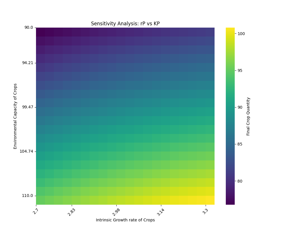
'''# 绘制热力图
plt.figure(figsize=(10, 8))
sns.heatmap(final_crops, xticklabels=5, yticklabels=5, cmap='viridis', cbar_kws={'label': 'Final Crop Quantity'})# 设置刻度标签
xticks_positions = np.linspace(0, len(rP_values) - 1, 5).astype(int)
yticks_positions = np.linspace(0, len(kP_values) - 1, 5).astype(int)
plt.xticks(xticks_positions, np.round(rP_values[xticks_positions], 2), rotation=45)
plt.yticks(yticks_positions, np.round(kP_values[yticks_positions], 2), rotation=0)# 添加标题和轴标签
plt.xlabel('Intrinsic Growth rate of Crops')
plt.ylabel('Environmental Capacity of Crops')
plt.title('Sensitivity Analysis: rP vs KP')plt.show()# 参数范围
kP_values = np.linspace(kP * 0.9, kP * 1.1, 20) # kP 在 ±10% 的范围
dP_values = np.linspace(0.01, 0.1, 20) # dP 自然死亡率在 0.01 到 0.1 范围# 创建网格
kP_grid, dP_grid = np.meshgrid(kP_values, dP_values)# 初始化存储最终结果的数组
final_crops_kP_dP = np.zeros_like(kP_grid)# 遍历参数网格
for i in range(kP_grid.shape[0]):for j in range(kP_grid.shape[1]):kP = kP_grid[i, j] # 当前 kPdP = dP_grid[i, j] # 当前 dP# 重置种群初始值P[:] = P0G[:] = G0I[:] = I0I2[:] = I20S[:] = S0F[:] = F0# 模拟模型for t in range(1, time_steps):DP = P0_func(t) - cG * G[t-1] * P[t-1] - bI2 * I2[t-1] * P[t-1] - dP * P[t-1]G[t] = G[t-1] + G0_func(t) * dt / 5P[t] = P[t-1] + DP * dt / 5# 记录最终作物数量final_crops_kP_dP[i, j] = P[-1]# 保存热力图数据
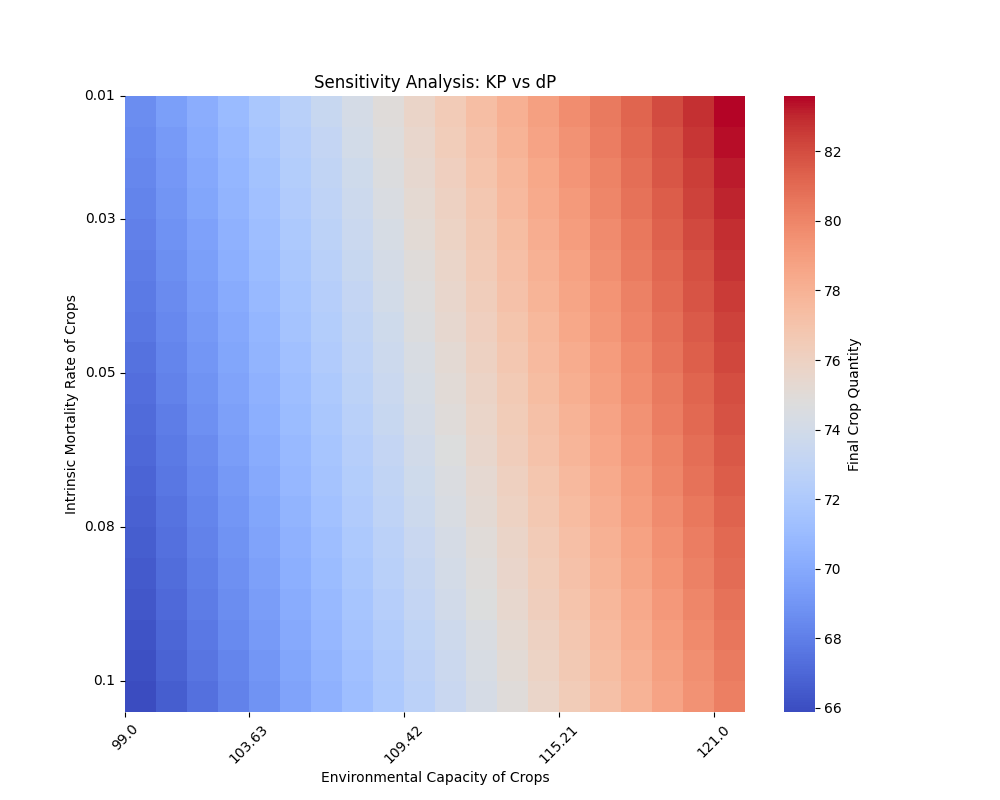
np.savez('kP_vs_dP_data.npz', kP_grid=kP_grid, dP_grid=dP_grid, final_crops=final_crops_kP_dP)# 绘制热力图
plt.figure(figsize=(10, 8))
sns.heatmap(final_crops_kP_dP, xticklabels=5, yticklabels=5, cmap='coolwarm', cbar_kws={'label': 'Final Crop Quantity'})
xticks_positions = np.linspace(0, len(kP_values) - 1, 5).astype(int)
yticks_positions = np.linspace(0, len(dP_values) - 1, 5).astype(int)
plt.xticks(xticks_positions, np.round(kP_values[xticks_positions], 2), rotation=45)
plt.yticks(yticks_positions, np.round(dP_values[yticks_positions], 2), rotation=0)
plt.xlabel('Environmental Capacity of Crops')
plt.ylabel('Intrinsic Mortality Rate of Crops')
plt.title('Sensitivity Analysis: KP vs dP')
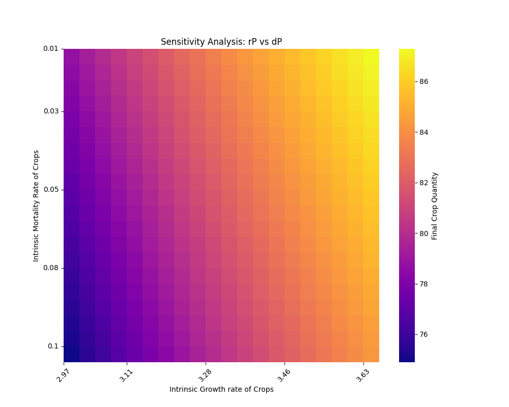
plt.show()# 参数范围
rP_values = np.linspace(rP * 0.9, rP * 1.1, 20) # rP 在 ±10% 的范围
dP_values = np.linspace(0.01, 0.1, 20) # dP 自然死亡率在 0.01 到 0.1 范围# 创建网格
rP_grid, dP_grid = np.meshgrid(rP_values, dP_values)# 初始化存储最终结果的数组
final_crops_rP_dP = np.zeros_like(rP_grid)# 遍历参数网格
for i in range(rP_grid.shape[0]):for j in range(rP_grid.shape[1]):rP = rP_grid[i, j] # 当前 rPdP = dP_grid[i, j] # 当前 dP# 重置种群初始值P[:] = P0G[:] = G0I[:] = I0I2[:] = I20S[:] = S0F[:] = F0# 模拟模型for t in range(1, time_steps):DP = P0_func(t) - cG * G[t-1] * P[t-1] - bI2 * I2[t-1] * P[t-1] - dP * P[t-1]G[t] = G[t-1] + G0_func(t) * dt / 5P[t] = P[t-1] + DP * dt / 5# 记录最终作物数量final_crops_rP_dP[i, j] = P[-1]# 保存热力图数据
np.savez('rP_vs_dP_data.npz', rP_grid=rP_grid, dP_grid=dP_grid, final_crops=final_crops_rP_dP)# 绘制热力图
plt.figure(figsize=(10, 8))
sns.heatmap(final_crops_rP_dP, xticklabels=5, yticklabels=5, cmap='plasma', cbar_kws={'label': 'Final Crop Quantity'})
xticks_positions = np.linspace(0, len(rP_values) - 1, 5).astype(int)
yticks_positions = np.linspace(0, len(dP_values) - 1, 5).astype(int)
plt.xticks(xticks_positions, np.round(rP_values[xticks_positions], 2), rotation=45)
plt.yticks(yticks_positions, np.round(dP_values[yticks_positions], 2), rotation=0)
plt.xlabel('Intrinsic Growth rate of Crops')
plt.ylabel('Intrinsic Mortality Rate of Crops')
plt.title('Sensitivity Analysis: rP vs dP')
plt.show()


